1. Create a List Box From a Range
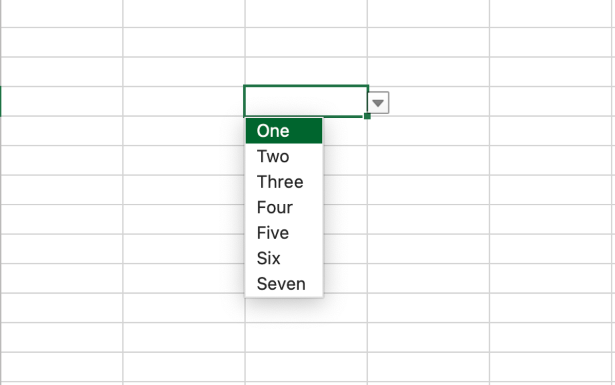
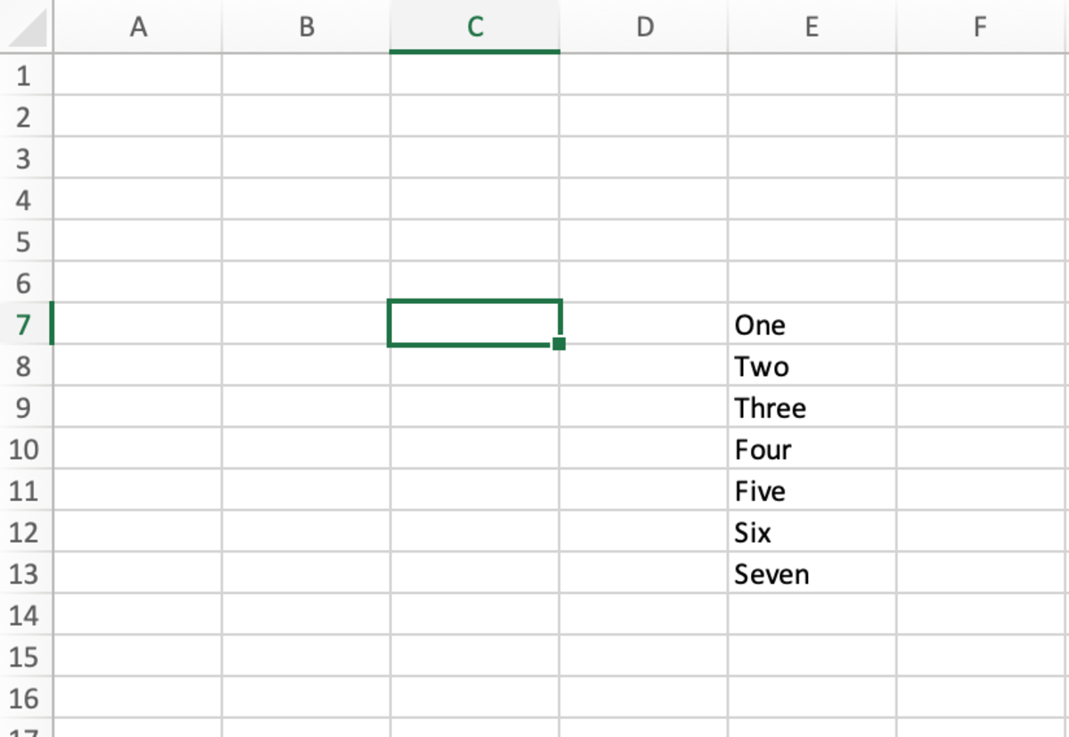
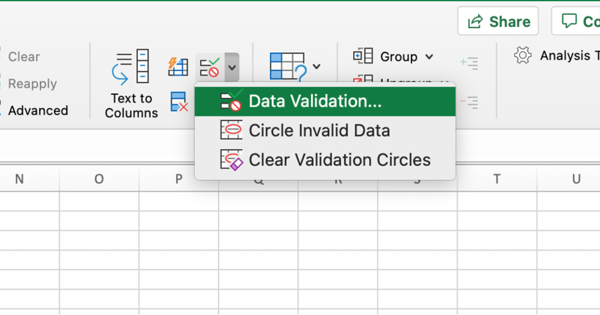
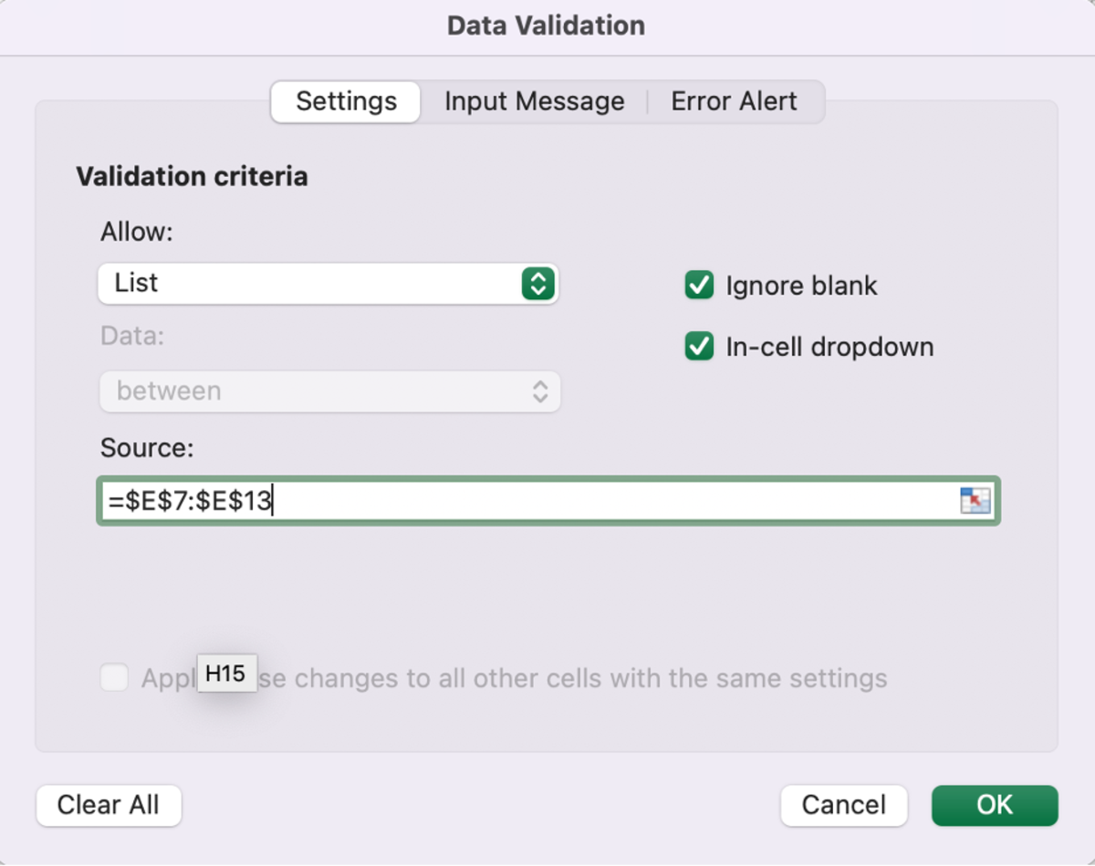
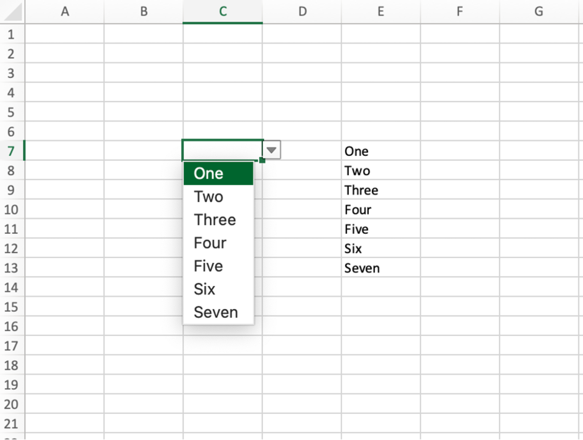
One of the easiest ways to create a list box is from a range of values. The range of cells used can be vertical like the one in the illustration or it can also be horizontal. First, select the cell(s) where you like the list box to appear. Next, select the data tab in the Excel ribbon, followed by clicking on the data validation option. A few options will appear in the data validation window. Select the list option under the allow and add the cell range of the list to the option to the source. After selecting OK, the list box will appear in the cell selected at the beginning of the process.
2. Create a List Box From a Named Range
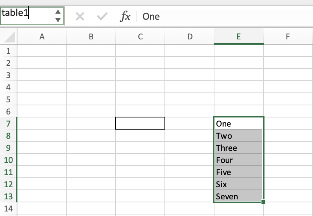
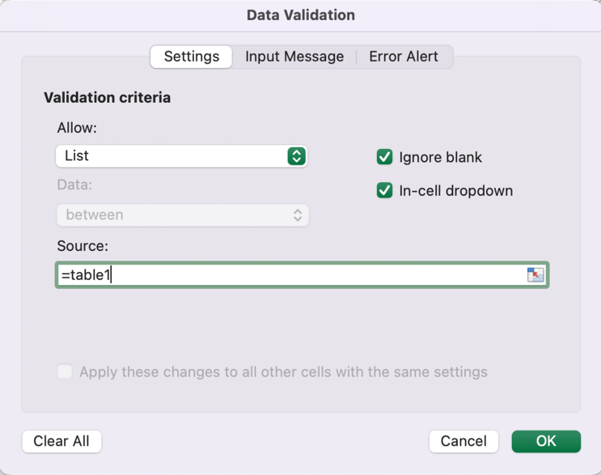
Like using a range, you may want your list to come from a named range. This option may be preferred if cell references for a list are expected to expand in the future. Using a named range will allow you to insert new cells into the named range without having to change a range in the source. To save the list as a named range, select the range of values and create a name in the reference field box shown in the upper left-hand corner of the below illustration. Next, tap on the enter key, and the range will be saved. As instructed earlier, select the cell(s) where you like the list box to appear. Select the data tab in the Excel ribbon, followed by clicking on the data validation option. Lastly, type the name of the range followed by clicking the OK button. The same result as the first option will appear.
3. Create a List Box Created With Hidden Values
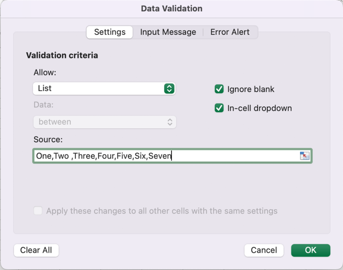
This option can be used when you don’t want the values In the list to be seen or easily edited in the spreadsheet. Under the data validation section, add each value to appear in the list box to the source section. Separate each value by a comma. This result will also be the same as the first two options. This content is accurate and true to the best of the author’s knowledge and is not meant to substitute for formal and individualized advice from a qualified professional. © 2022 Joshua Crowder

